Data Augmentation Methods in Time Series Forecasting
From frequency-domain perturbations to time–frequency wavelets, and finally to patch-based augmentation.
Data augmentation is a standard and often necessary component of modern machine learning pipelines. In computer vision, it is difficult to train a competitive model without it, and in time series classification a well-established body of techniques exists, including jittering, scaling, window slicing, time warping, permutation, rotation, and several pattern-based variants [1, 11, 12]. Time series forecasting, however, poses a fundamentally different problem.
In forecasting, the target is not a discrete class label but a continuous segment of the same signal that immediately follows the input. This distinction changes the nature of the task. A transformation that is safe for classification—such as warping part of the input or injecting noise into a window—can easily disrupt the relationship between the look-back window and the forecast horizon. When this relationship is broken, the model is trained on input–target pairs that are no longer mutually consistent, and predictive performance degrades accordingly.
Empirically, most classical augmentation methods that perform well in classification have been evaluated for forecasting and have largely failed to improve upon a no-augmentation baseline [2, 9]. This result is informative: it reveals an inherent tension in forecasting augmentation. The method must introduce sufficient diversity, so that the model observes variation beyond the raw training data, while simultaneously preserving temporal coherence, so that the augmented signal remains a valid continuous sequence. Reconciling these two requirements is what makes forecasting augmentation a distinctive and non-trivial problem.
Why classification-oriented augmentations struggle in forecasting
Many classical augmentation techniques—jittering, scaling, window warping, permutation—were originally designed for classification [11, 12]. They perform well when a transformation leaves the label unchanged. In forecasting, however, the "label" is the subsequent segment of the sequence. Perturbing only the input, warping a portion of the signal, or distorting local timing too aggressively produces an input whose corresponding future is no longer plausible. Chen et al. [2] evaluated these methods systematically and concluded that they generally fail to outperform models trained without augmentation.
Both the WaveMask/WaveMix work [8] and the TPS paper [13] emphasize the same point: forecasting demands a far stricter notion of input–target consistency than classification or anomaly detection. Randomness can be introduced, but it must be the correct kind of randomness—randomness that does not violate the temporal structure of the signal.
Data–label coherence: a necessary requirement
Let the look-back window be \(x\) and the forecast target be \(y\). Training operates over the continuous sequence \(s = x \Vert y\), not over \(x\) in isolation. Consequently, augmentation should act on the concatenated sequence and only afterwards be partitioned into input and target:
Although conceptually simple, this is one of the central ideas in forecasting augmentation. If augmentation is applied only to \(x\) while leaving \(y\) untouched, the natural continuity between input and target is broken. The TPS ablation studies [13] show that removing data–label coherence causes the largest performance degradation among all ablations considered.
Figure 1. The forecasting augmentation pipeline: the look-back window and forecast horizon are concatenated prior to augmentation and split afterwards, thereby preserving input–target alignment. (Figure adapted from [13].)
A taxonomy of forecasting augmentation methods
In recent years, the strongest augmentation methods for forecasting have come primarily from the frequency domain, from signal decomposition, or from carefully controlled signal-level manipulation. A concise taxonomy is as follows:
- Frequency-based: RobustTAD [3], FreqMask, FreqMix [2], WaveMask, WaveMix [8], Dominant Shuffle [9].
- Decomposition-based: STAug [4].
- Other methods: wDBA [6], MBB [7], Upsample [5].
- Patch-based: TPS [13].
The following sections review each family in turn, beginning with frequency-based methods, which have represented the dominant paradigm until recently.
RobustTAD
One of the foundational approaches in frequency-domain augmentation is RobustTAD [3]. The method first applies the discrete Fourier transform to the concatenated input sequence and forecast target, then perturbs selected frequency segments before transforming the sequence back to the time domain. In practice, the spectrum is treated as a combination of real and imaginary components, from which amplitude and phase information are derived.
Augmentation is performed by choosing a segment length proportionally to the full spectrum and modifying only those selected regions. In the amplitude-based version, the original magnitudes are replaced with values drawn from a Gaussian distribution controlled by a perturbation strength. In the phase-based version, the selected phase values are shifted by a small controlled perturbation. Although the original RobustTAD paper focused on anomaly detection, later forecasting studies [2, 4, 9] have adopted the magnitude-perturbation variant for multivariate time series forecasting, and our experiments also include phase perturbation.
FreqMask and FreqMix
FreqMask and FreqMix [2] are among the most widely used frequency-domain augmentations for forecasting. Both begin by concatenating input and target and applying the real FFT:
FreqMask zeroes out selected frequency components via a binary mask \(M\):
The underlying intuition is that suppressing selected periodic components encourages the model to be robust to their absence. FreqMix extends this idea by blending the spectra of two different sequences:
This allows one sequence to partially adopt the structural characteristics of another. Both methods are conceptually clean and simple to implement.
Figure 2. FreqMask removes selected frequency components; FreqMix blends frequencies between two sequences. (Figure from [2].)
A notable limitation is that both methods operate purely in the Fourier domain and therefore capture which frequencies are present, but not where those frequencies occur in time. This distinction proves to be important.
Time–frequency localization: WaveMask and WaveMix
This limitation was the principal motivation for the WaveMask and WaveMix methods [8]. The Fourier transform provides excellent global frequency information but discards temporal localization. The Short-Time Fourier Transform (STFT) improves on this through local windows, but the window size is fixed. Wavelets are more flexible: they operate simultaneously at multiple resolutions, offering high temporal resolution for high-frequency events and high frequency resolution for low-frequency trends.
Figure 3. Time–frequency resolution comparison. The Fourier Transform has no time localization; the STFT uses fixed-size windows; the Wavelet Transform adapts its resolution across scales. (Figure adapted from [8, 16].)
A useful summary: the FFT describes which frequencies exist, whereas wavelets describe which frequencies exist and approximately where they occur. For time series data, where local changes frequently carry critical information, this additional localization is highly valuable.
In WaveMask/WaveMix [8], the signal is decomposed via the discrete wavelet transform (DWT) into approximation and detail coefficients across multiple levels. Augmentation then operates directly on those coefficients:
An important advantage is that masking and mixing can be applied independently at each decomposition level, so fine-scale detail and coarse-scale trends need not be treated identically. In the reported experiments, WaveMask and WaveMix outperform all baselines in 12 out of 16 forecasting horizon settings and rank second in the remaining four [8].
Figure 4. WaveMask pipeline: the signal is decomposed via DWT, wavelet coefficients are selectively masked at each level, and the signal is reconstructed via inverse DWT. (Figure from [8].)
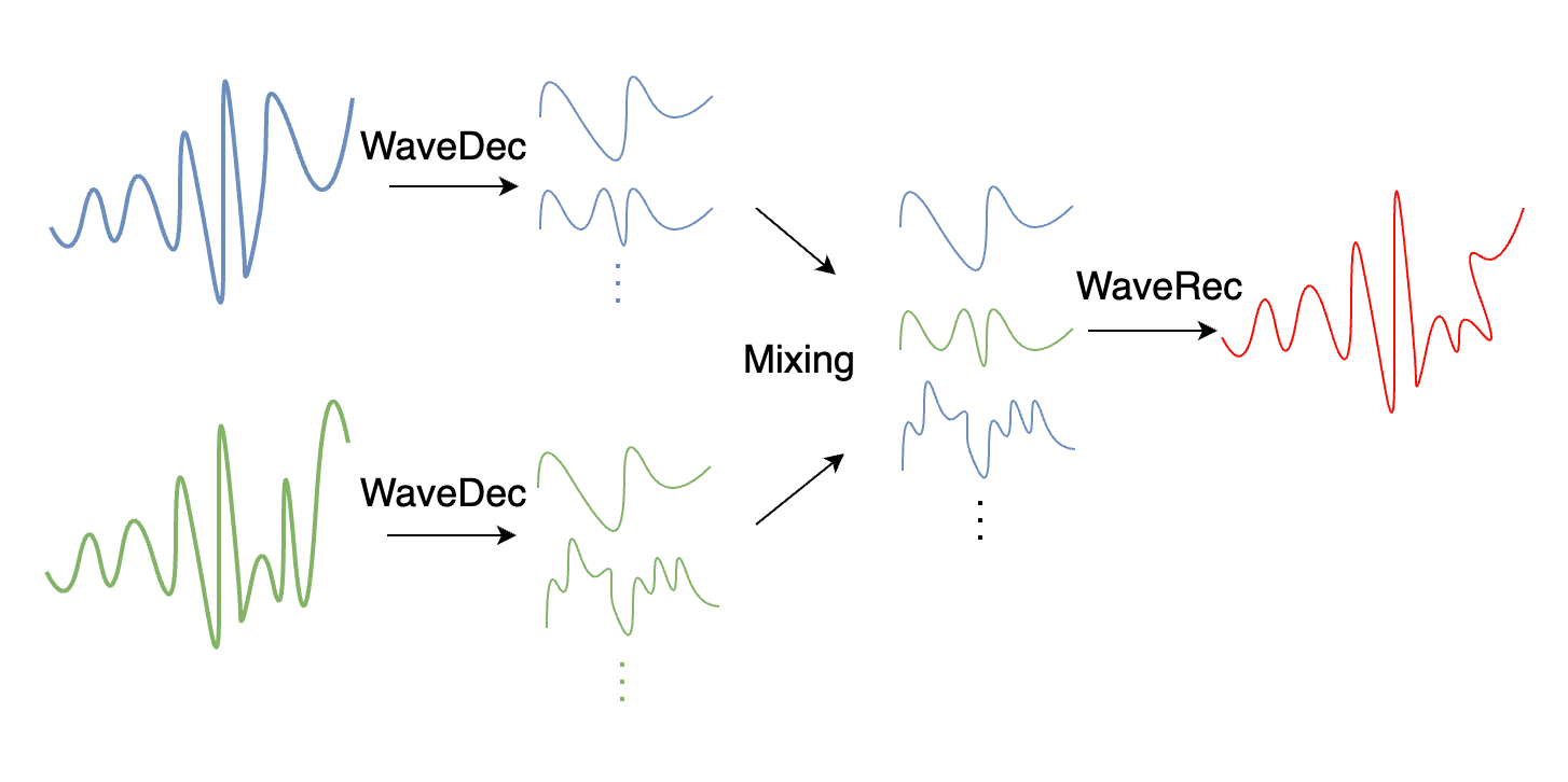
Figure 5. WaveMix pipeline: two signals are decomposed, their wavelet coefficients are exchanged via complementary masks, and the blended coefficients are reconstructed. (Figure from [8].)
Dominant Shuffle
Dominant Shuffle [9] adopts a more targeted approach to frequency-domain augmentation. Rather than masking or mixing arbitrary spectral components, it identifies the most dominant frequencies and shuffles them prior to reconstruction:
The underlying motivation is to avoid perturbing the entire spectrum too aggressively, which risks pushing augmented samples out of distribution—an issue discussed at length in the original paper. That said, in the unified comparisons reported in the TPS paper [13], Dominant Shuffle is not the strongest method overall.
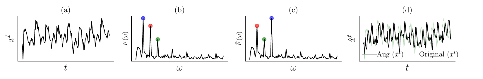
Figure 6. Dominant Shuffle: the top-\(k\) dominant frequency components are identified and shuffled, while the rest of the spectrum is left unchanged. (Figure from [9].)
STAug
STAug [4] originates from the decomposition-based family. It applies Empirical Mode Decomposition (EMD) to two sequences, yielding intrinsic mode functions (IMFs), and then recombines them using mixup-style interpolation weights drawn from a uniform distribution. The result is a new sequence that blends the temporal characteristics of both inputs.
Conceptually, STAug offers an elegant mechanism for producing diverse yet coherent samples. Its main practical limitation is computational cost: EMD is memory-intensive, particularly on larger datasets. In the TPS experiments [13], STAug could not be evaluated on the ECL and Traffic datasets due to GPU memory constraints—a limitation also acknowledged in the original STAug paper [4].
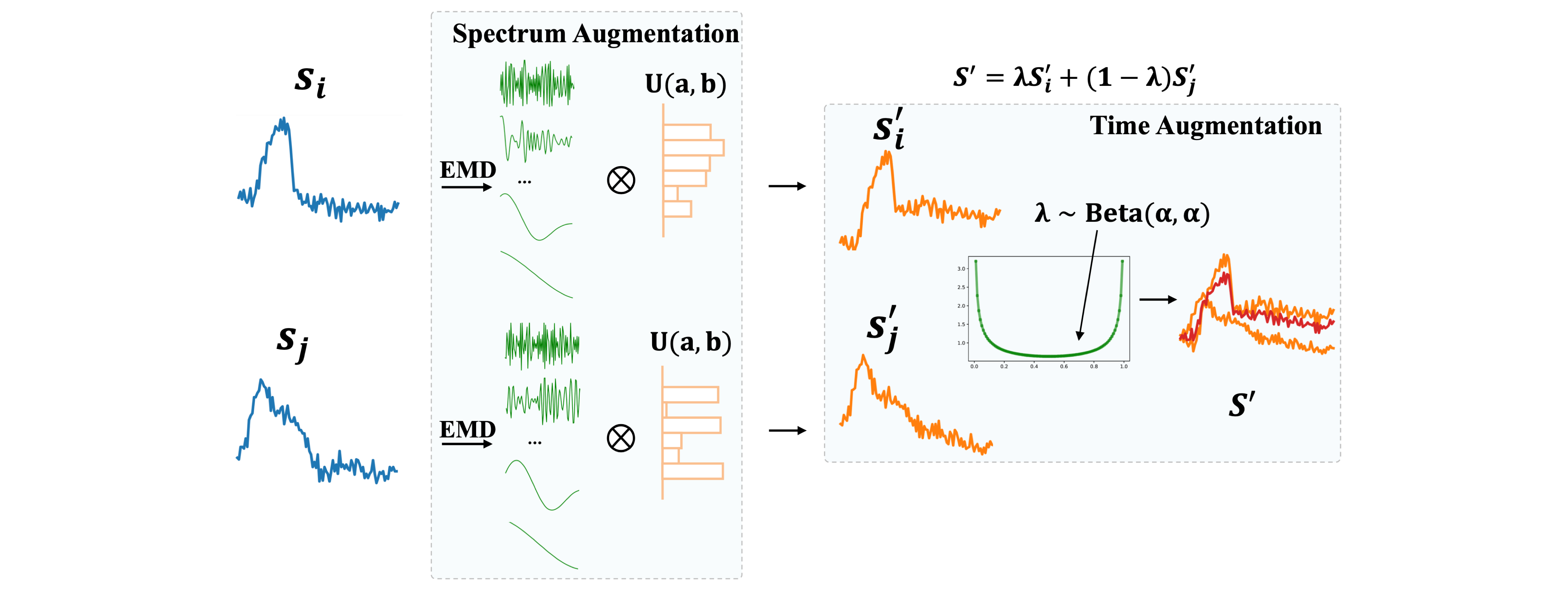
Figure 7. STAug decomposes two sequences via EMD into intrinsic mode functions (IMFs) and recombines them via interpolation weights. (Figure from [4].)
wDBA, MBB, and Upsample
These three methods are worth mentioning because they illustrate the breadth of the forecasting augmentation landscape beyond frequency-based approaches.
- wDBA [6] constructs new samples by averaging time series under DTW-based alignment. It produces clean synthetic data but carries substantial computational cost.
- MBB [7] decomposes a series into trend, seasonal, and remainder components via STL, then bootstraps blocks from the remainder to generate new sequences.
- Upsample [5] selects a consecutive segment and stretches it back to the original length using linear interpolation, acting as a magnifying-glass-like view of local structure.
Upsample is notable for consistently ranking among the stronger non-frequency baselines and often providing a competitive benchmark. Across the broader evaluation in the TPS paper [13], however, TPS performs better overall.
From image patches to temporal patches
Patch-based augmentation is a well-established tool in computer vision. Methods such as PatchShuffle [14] and PatchMix [15] divide an image into patches, apply shuffling or mixing, and reassemble the image. These methods exploit the spatial redundancy of images: local pixel rearrangements within patches generally preserve the overall scene.
Time series are fundamentally different. They are sequential in nature, and the order of values carries meaning at every scale. Naively cutting a sequence into non-overlapping chunks and shuffling them would create hard boundaries, visible discontinuities, and input–target misalignment. Transferring the patch-based idea to the temporal domain therefore requires careful rethinking of each step.
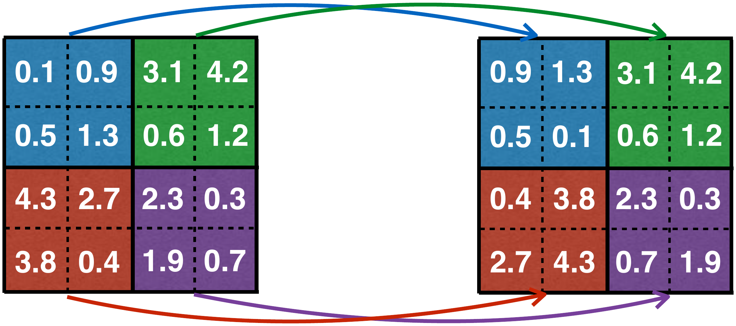
Figure 8. PatchShuffle in computer vision: a 4×4 image is partitioned into non-overlapping 2×2 patches, and pixels within each patch are independently shuffled. (Figure adapted from [13] and [14].)
Temporal Patch Shuffle (TPS)
TPS [13] is the method developed to address these challenges. Its core procedure is as follows. Given the full sequence (the concatenation of look-back window and forecast horizon), TPS extracts overlapping temporal patches, computes a variance-based score for each patch, selectively shuffles a subset of patches—prioritizing low-variance patches—and reconstructs the sequence by averaging over the overlapping regions.
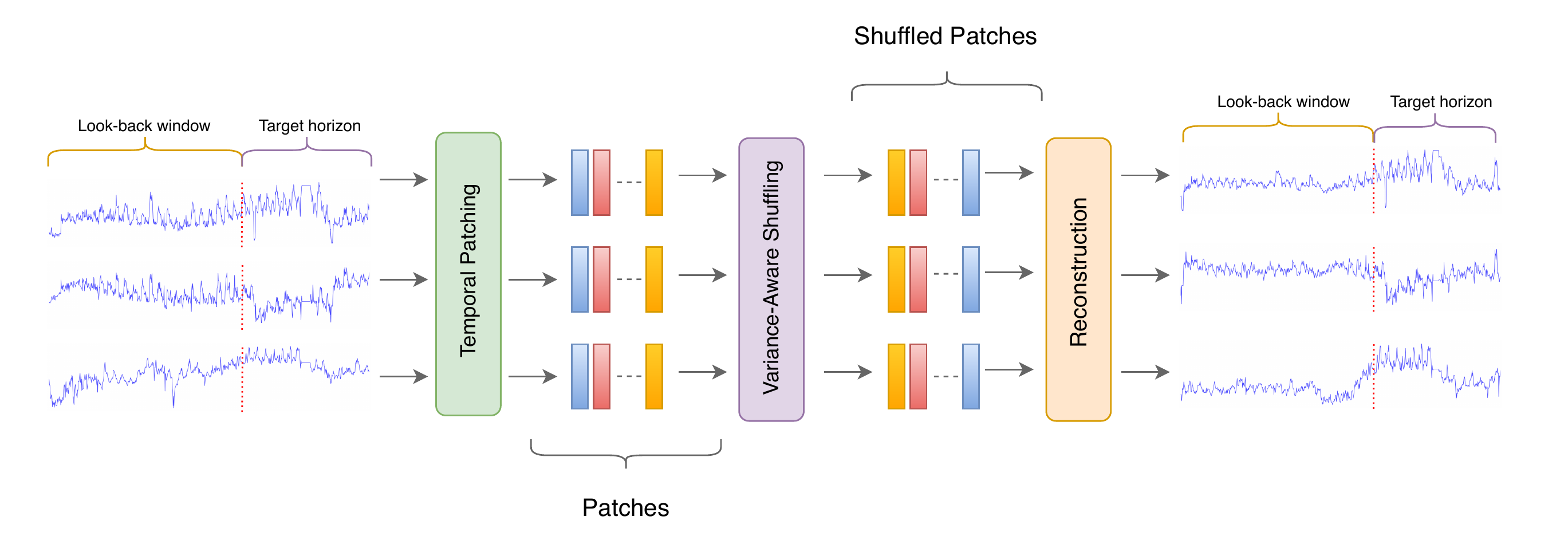
Figure 9. TPS pipeline. The input sequence is partitioned into overlapping patches (Temporal Patching); a subset is reordered according to variance scores (Variance-Aware Shuffling); and the sequence is reconstructed by averaging overlapping regions (Reconstruction). (Figure from [13].)
Procedure
The full procedure, as specified in the paper [13], consists of the following steps:
- Concatenate. Join the look-back window and forecast horizon into a single continuous sequence. This enforces data–label coherence from the outset.
- Temporal Patching. Extract overlapping patches using patch length \(p\) and stride \(s\). Overlap is essential: neighboring patches share time steps, which smooths transitions during reconstruction.
- Variance scoring. Compute the variance of each patch across all channels in the normalized input space. Low-variance patches are treated as safer to perturb, as they contain less distinctive structure—a conservative heuristic.
- Selective shuffling. Select the fraction \(\alpha\) of lowest-variance patches and randomly permute their positions; the remaining patches are left untouched.
- Reconstruction. Place each patch back at its (possibly new) temporal position and average over overlapping regions. Averaging serves as a natural smoothing mechanism that softens any discontinuities introduced by shuffling.
- Split. Separate the reconstructed sequence back into augmented input and augmented target.
Formally, the algorithm is as follows [13]:
Ensure: augmented sequence S
- X ← [L, F] # X ∈ ℝB×T×C
- P ← Unfold(X, p, s) # P ∈ ℝB×Np×C×p
- Score ← Var(P) # ℝB×Np
- Ns ← ⌊\(\alpha\)Np⌋
- for b = 0 to B − 1 do
- Ib ← Argsort(Score[b, :])[0 : Ns]
- \(\pi_b\) ← RandPerm(Ns)
- Pb[Ib] ← Pb[Ib][\(\pi_b\)]
- end for
- \(\tilde{P}\) ← P # shuffled patch tensor
- S ← Reconstruct(\(\tilde{P}\))
Three hyperparameters control the method: the patch length \(p\), the stride \(s\), and the shuffle rate \(\alpha\). In practice, these are selected through a validation-based search over a predefined set of candidate combinations (approximately 20 configurations), rather than a full Cartesian grid [13].
Ablation findings
The ablation studies in the TPS paper [13] isolate the contribution of each design choice. The findings, roughly ordered by importance, are as follows.
- Data–label coherence matters the most. Applying augmentation only to the input while leaving the target unchanged causes the largest performance drop of any single ablation. This empirically confirms the central thesis: in forecasting, input and target must be transformed jointly.
- Overlap matters substantially. Replacing overlapping patches with non-overlapping ones leads to a clear degradation. Overlap is the mechanism that preserves local temporal structure under shuffling.
- Variance-based ordering provides a modest improvement. Its effect is smaller than overlap, but it remains a useful refinement when only a subset of patches is shuffled. When \(\alpha = 1.0\) (all patches shuffled), variance ordering becomes irrelevant by construction.
- The time domain outperforms the frequency domain. A variant that applies the same patch operations after an FFT transform also degrades results, indicating that TPS is most effective when operating directly on the raw time-domain signal.
- Higher shuffle rates tend to help. In the sensitivity study, values in the range 0.7–1.0 consistently yield the strongest results across datasets.
Main results
Long-term forecasting
TPS was evaluated on nine long-term forecasting datasets using five recent backbone families: TSMixer, DLinear, PatchTST, TiDE, and LightTS. Across all backbones, TPS achieves the best average MSE among the compared augmentation methods [13]. The figure below summarizes the comparison.
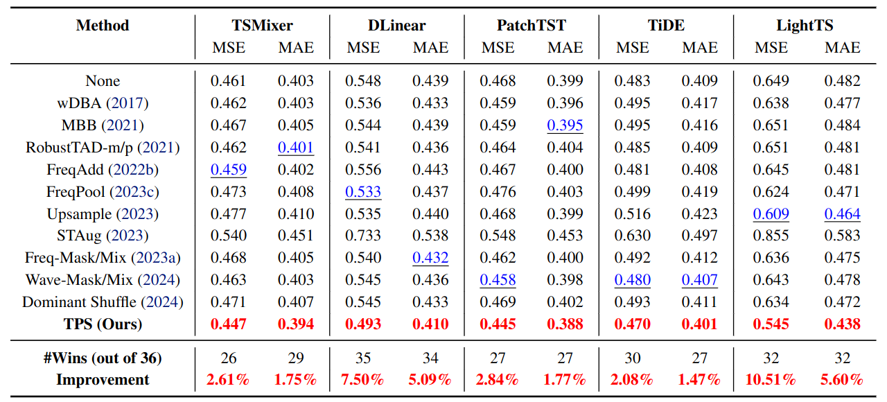
Figure 10. Long-term forecasting results across nine datasets and five backbones. TPS achieves the best average MSE and the highest number of wins for every backbone. Across the five backbones, relative MSE improvements over the best competing augmentation range from 2.08% to 10.51%. (Results from [13]; see the paper for per-dataset tables.)
The improvement for LightTS (10.51%) is the largest, but the broader narrative is one of consistency: TPS does not rely on a single favorable backbone or dataset. It yields gains across architectures ranging from linear models (DLinear, LightTS) to MLP-based designs (TSMixer, TiDE) and transformer-style models (PatchTST).
Short-term traffic forecasting
TPS was further evaluated on four short-term traffic datasets (PeMS-03, 04, 07, 08) using PatchTST, again achieving the strongest overall augmentation performance [13].
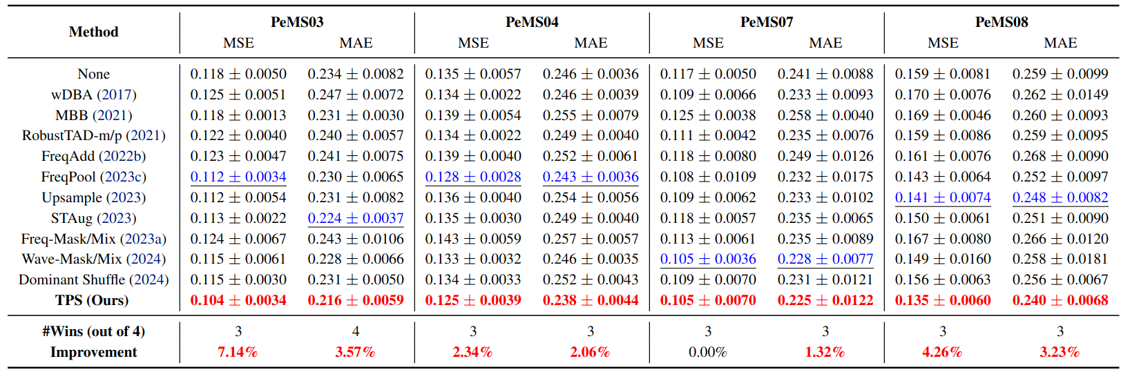
Figure 11. Short-term traffic forecasting results with PatchTST on PeMS-{03, 04, 07, 08}. TPS achieves MSE improvements of 7.14%, 2.34%, 0.00%, and 4.26% respectively over the best competing augmentation. Even where the gain is small (PeMS07), TPS does not degrade performance. (Results from [13].)
Stability matters as much as peak performance: a good augmentation method should not behave like a lottery ticket, producing large gains on some datasets and substantial losses on others.
Extension to time series classification
One particularly appealing aspect of TPS is how naturally it transfers to classification. Since classification tasks do not have a forecast horizon, only two modifications are required: operate on the input sequence \(X\) directly (without concatenation), and apply shuffling at the sample level rather than the batch level. With these minimal changes, TPS achieves the best average accuracy among compared augmentation methods on both univariate (UCR) and multivariate (UEA) benchmarks [13].
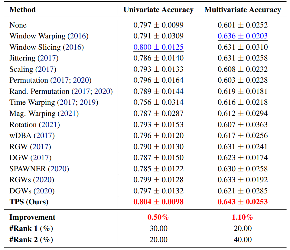
Figure 12. Classification results. On 30 UCR univariate datasets (MiniRocket), TPS improves accuracy by 0.50% over the best competing method, with top-2 placement on 50% of datasets. On 10 UEA multivariate datasets (MultiRocket), TPS improves accuracy by 1.10%, with top-2 placement on 60% of datasets. (Results from [13].)
This provides encouraging evidence that the core patch-based idea generalizes beyond forecasting.
Summary
Taken together, TPS stands out for a combination of reasons. It avoids expensive decomposition steps, does not indiscriminately alter the entire spectrum, and does not break the input–target relationship. Instead, it modifies the sequence in a controlled manner, with overlap and averaging preserving local temporal structure and data–label coherence keeping input and target aligned.
Across evaluations, TPS achieves state-of-the-art augmentation performance on long-term forecasting (nine datasets, five backbones), short-term forecasting (four PeMS traffic datasets), and time series classification (UCR and UEA benchmarks). This breadth across tasks and architectures is what makes the approach particularly promising.
Future directions
The TPS paper [13] outlines several directions for future work:
- Broader backbone coverage. Evaluating TPS with additional model families, including Graph Neural Networks and Spiking Neural Networks, as well as newer foundation-model settings under lightweight adaptation protocols such as frozen-backbone fine-tuning.
- More expressive patch-importance criteria. Replacing the variance-based ordering with channel-aware or weighted multivariate scoring, which could better reflect the relative informativeness of patches in high-dimensional settings.
- Cold-start forecasting. Evaluating TPS in low-data regimes, where only a small fraction (e.g., 10% or 20%) of the training data is available—a setting explored in prior work [2].
- Standardized benchmark suites. Applying TPS to standardized long-horizon benchmarks such as GIFT-Eval, to further stress-test the method in large-scale evaluations.
As a preliminary indication of the first point, the TPS paper additionally reports results on CycleNet—a recent state-of-the-art forecasting backbone—where TPS also outperforms all competing augmentation methods, with a 1.74% improvement over the second-best method on ETTh1.
References
- Wen, Q., Sun, L., Yang, F., Song, X., Gao, J., Wang, X., Xu, H. (2021). Time Series Data Augmentation for Deep Learning: A Survey. IJCAI 2021.
- Chen, M., Xu, Z., Zeng, A., Xu, Q. (2023). FrAug: Frequency Domain Augmentation for Time Series Forecasting. arXiv:2302.09292.
- Gao, J., Song, X., Wen, Q., Wang, P., Sun, L., Xu, H. (2021). RobustTAD: Robust Time Series Anomaly Detection via Decomposition and Convolutional Neural Networks. arXiv:2002.09545.
- Zhang, X., Chowdhury, R. R., Shang, J., Gupta, R., Hong, D. (2023). Towards Diverse and Coherent Augmentation for Time-Series Forecasting. arXiv:2303.14254.
- Semenoglou, A.-A., Spiliotis, E., Assimakopoulos, V. (2023). Data Augmentation for Univariate Time Series Forecasting with Neural Networks. Pattern Recognition, 134:109132.
- Forestier, G., Petitjean, F., Dau, H. A., Webb, G. I., Keogh, E. (2017). Generating Synthetic Time Series to Augment Sparse Datasets. IEEE ICDM 2017.
- Bandara, K., Hewamalage, H., Liu, Y.-H., Kang, Y., Bergmeir, C. (2021). Improving the Accuracy of Global Forecasting Models Using Time Series Data Augmentation. Pattern Recognition, 120:108148.
- Arabi, D., Bakhshaliyev, J., Coskuner, A., Madhusudhanan, K., Uckardes, K. S. (2024). Wave-Mask/Mix: Exploring Wavelet-Based Augmentations for Time Series Forecasting. arXiv:2408.10951.
- Zhao, K., He, Z., Hung, A., Zeng, D. (2024). Dominant Shuffle: A Simple Yet Powerful Data Augmentation for Time-Series Prediction. arXiv:2405.16456.
- Iwana, B. K., Uchida, S. (2021). An Empirical Survey of Data Augmentation for Time Series Classification with Neural Networks. PLOS ONE, 16(7):1–32.
- Um, T. T., Pfister, F. M. J., et al. (2017). Data Augmentation of Wearable Sensor Data for Parkinson's Disease Monitoring Using Convolutional Neural Networks. ICMI 2017.
- Le Guennec, A., Malinowski, S., Tavenard, R. (2016). Data Augmentation for Time Series Classification Using Convolutional Neural Networks. ECML/PKDD Workshop.
- Bakhshaliyev, J., Burchert, J., Landwehr, N., Schmidt-Thieme, L. (2026). Temporal Patch Shuffle (TPS): Leveraging Patch-Level Shuffling to Boost Generalization and Robustness in Time Series Forecasting. arXiv:2604.09067.
- Kang, G., Dong, X., Zheng, L., Yang, Y. (2017). PatchShuffle Regularization. arXiv:1707.07103.
- Hong, Y., Chen, Y. (2024). PatchMix: Patch-Level Mixup for Data Augmentation in Convolutional Neural Networks. Knowledge and Information Systems, 66:3855–3881.
- Gabry, M. A., Eltaleb, I., Soliman, M. Y., Farouq-Ali, S. M. (2023). A new technique for estimating stress from fracture injection tests using continuous wavelet transform. Energies, 16(2), 764. https://www.mdpi.com/1996-1073/16/2/764.