Spiking Neural Networks for Time Series Forecasting
From Hodgkin–Huxley simplifications and LIF dynamics, through CPG positional encodings and dual-compartment neuron models, and finally to graph-structured Fourier spectral operators for energy-efficient multivariate forecasting.
Spiking Neural Networks (SNNs) have emerged as an energy-efficient alternative to conventional neural networks. Instead of transmitting continuous-valued activations at every layer, SNNs communicate through sparse binary spike events. This event-driven view makes them attractive for resource-constrained settings and neuromorphic hardware, where computation can be performed only when spikes occur.
For a long time, most successful SNN applications were in computer vision, event-based sensing, robotics, and other domains where sparse events are natural. More recently, SNNs have started to appear in time series forecasting (TSF). This direction is promising because forecasting is inherently temporal: the model has to understand how a signal evolves over time. At the same time, TSF is challenging for SNNs because real-world time series are continuous-valued, while SNNs work with discrete spikes. Therefore, successful SNN forecasting models need careful temporal alignment, effective spike encoding, and architectures that can model both short-term and long-term patterns.
This blog gives an overview of this development. We start from basic neuron models, introduce the Leaky Integrate-and-Fire (LIF) neuron used in many forecasting models, discuss temporal alignment, then move through the main SNN forecasting directions: spiking TCN/RNN/Transformer backbones, CPG-based positional encoding, Temporal Segment LIF neurons, SpikF, and finally SpikF-GO, our graph-based spiking Fourier model for multivariate time series forecasting.
From Biological Neuron Models to SNNs
The idea of using spikes as computational signals is not new. Maass described networks of spiking neurons as the third generation of neural network models, after threshold-based networks and continuous activation-based neural networks [1]. The important change is that the timing of spikes becomes part of the computation. A neuron does not only say how much it is activated; it also says when it fires.
A biological neuron is a complex dynamical system. The Hodgkin–Huxley model is one of the classical detailed models for action potential generation. It describes the membrane current using the membrane capacitance and ionic currents, especially sodium, potassium, and leak currents [4]. In a simplified form, the membrane current can be written as:
This model is biologically meaningful, but it is also mathematically and computationally more expensive than what we usually want inside deep learning models. For this reason, most SNN forecasting models use simpler neuron models. The most common one is the Leaky Integrate-and-Fire neuron. It keeps the main idea of membrane potential accumulation, leakage, threshold crossing, spike emission, and reset, but it avoids the detailed ion-channel dynamics of Hodgkin–Huxley.
The general SNN literature also shows why this simplification is useful. SNNs can exploit sparsity, temporal coding, and event-driven processing, and they are especially suitable for neuromorphic hardware. Review papers report applications in computer vision, robotics, motor control, navigation, biosignal processing, and other low-power settings [3].
The LIF Neuron and Surrogate Gradients
In the forecasting models discussed here, the LIF neuron is usually the fundamental spiking unit. In discrete time, we can write the membrane update as:
Here, \(U[t]\) is the membrane potential at step \(t\), \(I[t]\) is the input current from the previous layer, \(\beta < 1\) is the decay factor, \(\vartheta\) is the firing threshold, and \(V_{\mathrm{reset}}\) is the reset potential. When the membrane potential crosses the threshold, the neuron emits a binary spike \(S[t]=1\). Otherwise, no spike is emitted and the membrane potential decays.
The main difficulty is training. The spike function \(\mathbf{1}(\cdot)\) is non-differentiable, so standard backpropagation cannot pass gradients through it directly. A common solution is to use surrogate gradients during Backpropagation Through Time (BPTT) [2]. One practical choice is the arctangent surrogate:
where \(\alpha\) controls the sharpness of the approximation. This does not make the forward pass non-spiking: the model can still use binary spikes in the forward computation. The surrogate is mainly used to make the backward pass trainable.
Temporal Alignment for Time Series Forecasting
A key question in SNN forecasting is how to align a continuous time series with the discrete spiking dimension. A regular time series has a sampling interval \(\Delta T\), while an SNN simulation uses a smaller internal time step \(\Delta t\). A common solution is to divide each time-series step into \(T_s\) finer spiking steps:
This means that each time-series observation can be represented by multiple possible spike events. For an input with \(T\) time steps and \(N\) variables, the model can process up to \(T_s \times T \times N\) spike events per sample. A spike encoder then converts the original floating-point values into spike trains with temporal resolution \(T_s\).
This step is more important than it first appears. If the encoding is too simple, the model may lose meaningful information from the continuous signal. If the encoding is too dense, the model may lose the energy benefit of sparse spikes. Therefore, early SNN forecasting work focused not only on backbones, but also on spike encoders and temporal alignment.
Problem Formulation: Multivariate Time Series Forecasting
We follow the problem formulation used in our SpikF-GO paper. In multivariate time series forecasting, the goal is to predict future values of several correlated variables over time. A batch of multivariate time series with batch size \(B\), sequence length \(T\), and \(N\) variables is represented as:
where \(X_{b,t,n}\) denotes the value of variable \(n \in \{1,\ldots,N\}\) at time \(t \in \{1,\ldots,T\}\) for sample \(b \in \{1,\ldots,B\}\). We denote the \(N\)-dimensional observation vector at time \(t\) by \(x_{b,t} \in \mathbb{R}^{N}\).
Given a look-back window length \(L < T\) and a forecast horizon \(O = T-L\), the input window and prediction target for each sample \(b\) are constructed as:
Stacking all input windows and targets gives the batched tensors:
A forecasting model \(F_{\theta}\), parameterized by \(\theta\), learns the mapping:
The model is trained by minimizing Mean Squared Error over mini-batches:
where \(\lVert\cdot\rVert_F\) denotes the Frobenius norm. Although this formulation is simple, the modeling problem is not. A good multivariate forecasting model should learn temporal dependencies within each variable, dependencies between variables, and how these relationships change over time.
First Systematic SNN Forecasting Backbones
The first systematic study of SNNs for time series forecasting proposed spiking variants of common temporal backbones: Spike-TCN, Spike-RNN, Spike-GRU, and iSpikformer [5]. This work showed that SNNs can be competitive with classical ANN forecasting models while using much lower theoretical energy.
Spike-TCN
A Temporal Convolutional Network (TCN) models sequences with causal and dilated convolutions [12]. In the spiking version, standard activation functions such as ReLU are replaced by spiking neuron layers. Hardware-unfriendly operations such as dropout are removed, and residual connections are adapted to a spike-compatible form. Since TCNs do not carry recurrent states across time steps, the membrane state can be reset at the beginning of each time-series step, which makes parallel training easier.
Spike-RNN and Spike-GRU
RNNs are natural candidates for sequence modeling because they maintain an internal hidden state. In a Spike-RNN, the recurrent activation is replaced with a spiking neuron layer. Unlike Spike-TCN, the membrane potential is carried across time steps, which gives the model a stateful temporal memory. GRU-style gating can also be adapted to improve long-term dependency modeling [13].
iSpikformer
Transformers are powerful for time series, but attention has a known issue: without positional information, self-attention is permutation-invariant. iSpikformer adapts the inverted Transformer idea into a spiking architecture, showing that spike-based temporal processing can be combined with modern spatial modeling across variables.
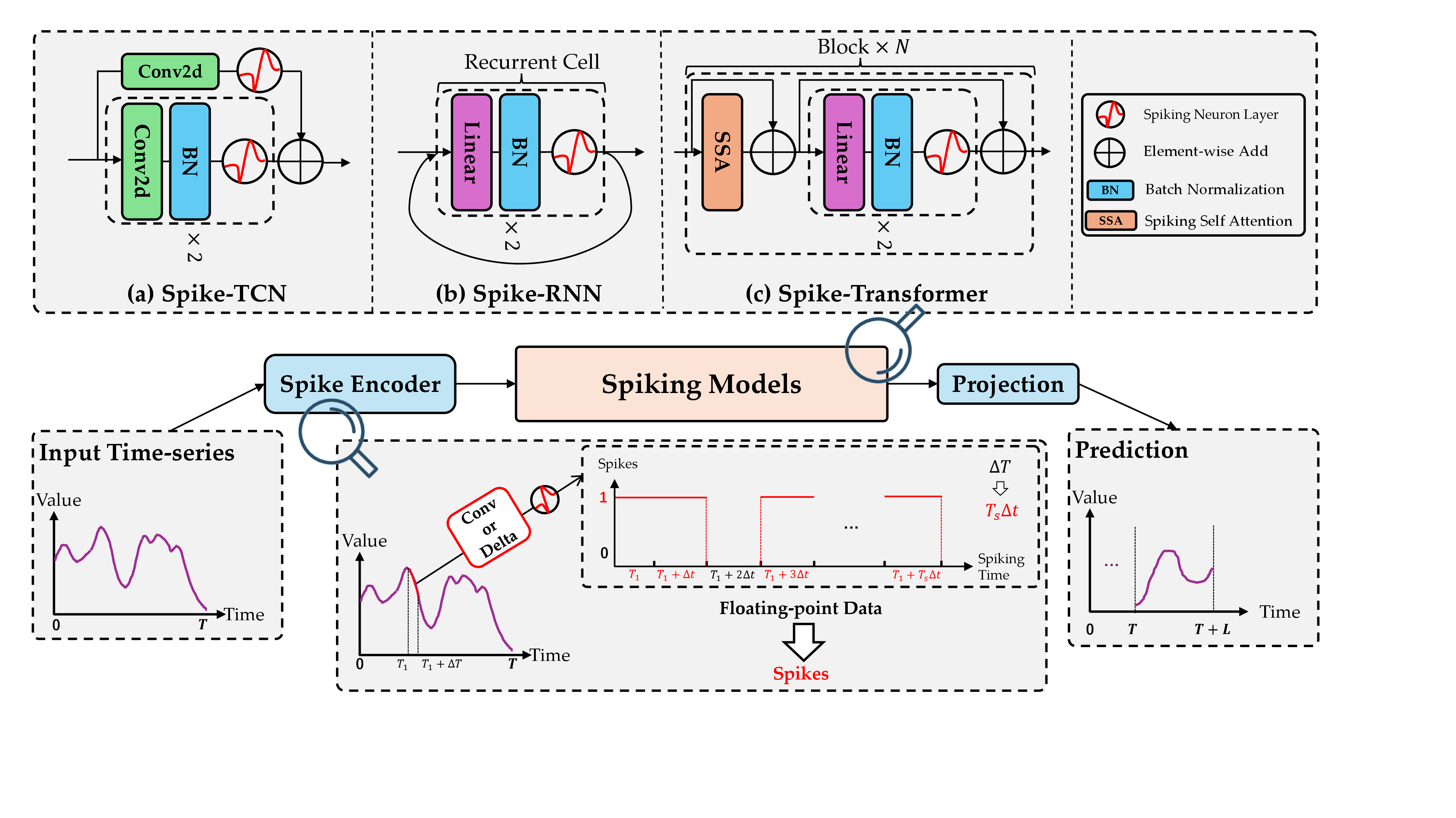
Figure 1. Spiking forecasting backbones from the first systematic SNN forecasting framework. The pipeline converts continuous time-series values into spike trains, processes them with spike-compatible TCN, recurrent, and Transformer-style architectures, and decodes the spike features back to continuous forecasts.
The main result from this line of work is that SNNs are not only biologically inspired. They can also be practical forecasting models. On the Electricity benchmark, the study reported a theoretical energy reduction of 63.60% for Spike-TCN compared to TCN, 75.05% for Spike-GRU compared to GRU, and 66.30% for iSpikformer compared to iTransformer [5]. This made SNN forecasting a realistic research direction rather than only a conceptual idea.
CPG-Based Positional Encoding
A second direction focuses on positional information. Sequence models need to know the order of input elements. This is easy to handle in standard Transformers with sinusoidal or learned positional embeddings, but it is harder in SNNs because the representation should remain spike-based and hardware-friendly.
Central Pattern Generators (CPGs) are biological neural circuits that produce rhythmic patterned outputs without requiring rhythmic inputs. Inspired by this mechanism, CPG-PE proposes a spike-form positional encoding strategy for SNNs [6]. The key observation is that sinusoidal positional encoding can be interpreted as a special solution of a simple CPG-like dynamical system.
The output is still binary, because a spike is emitted only when the sinusoidal membrane signal exceeds the threshold. Instead of adding positional encodings to spike matrices, CPG-PE concatenates the positional spike matrix with the input spike matrix, then maps the dimension back using a linear layer, batch normalization, and a spiking neuron layer. This avoids producing non-binary values from direct addition.
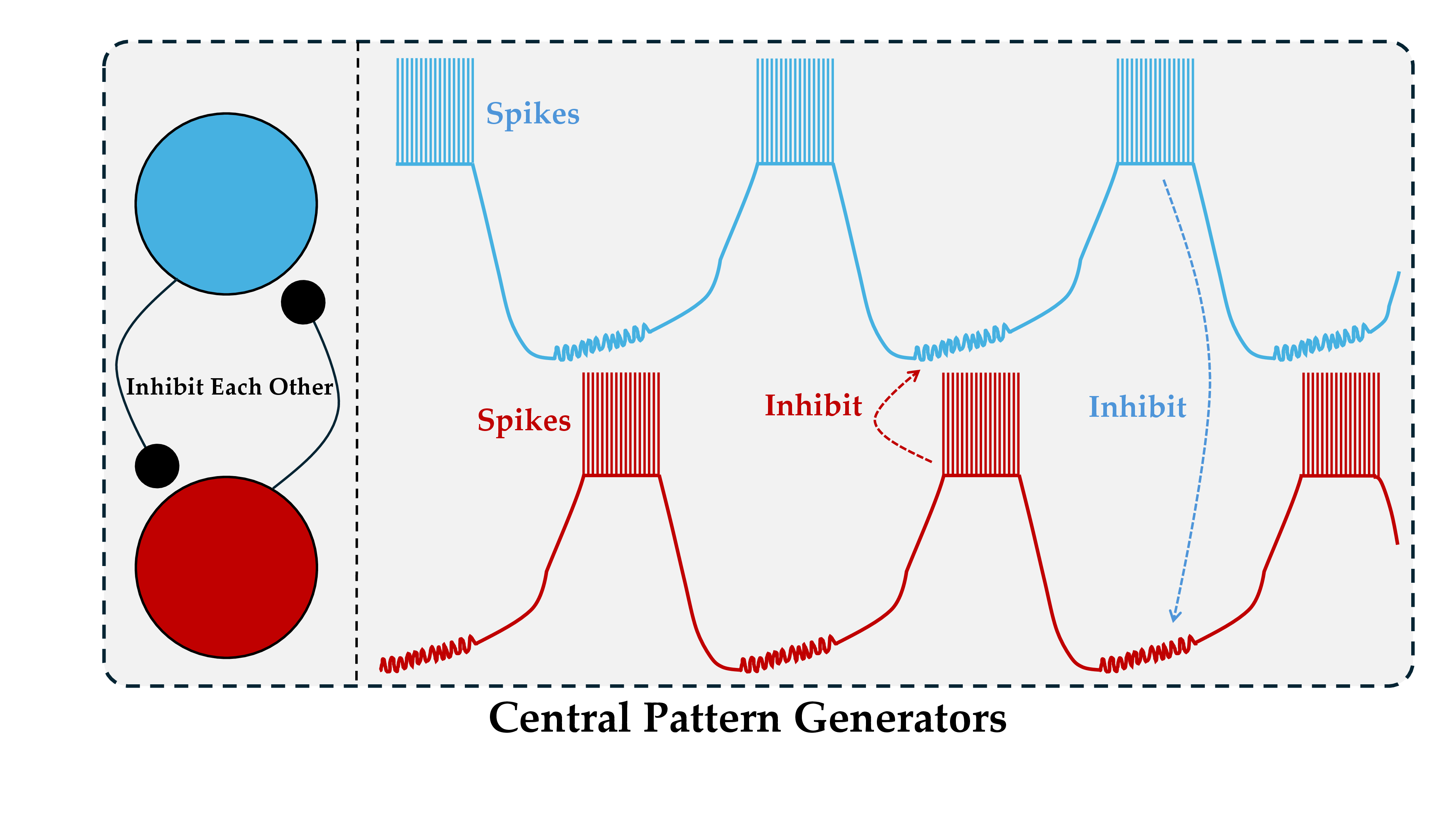
Figure 2. CPG-based positional encoding for SNNs. CPG neurons generate binary rhythmic spike patterns that encode sequence position; the positional spike matrix is concatenated with the input spike matrix and mapped back to the original feature dimension.
In time series forecasting, CPG-PE improved spiking TCN, RNN, and Transformer models. The reported average improvement was \(+0.013\) in \(R^2\) and \(-0.022\) in RSE compared to SNNs without positional encoding [6]. This suggests that position remains an open and important issue in spiking sequence models.
Improving the Neuron: Temporal Segment LIF
Another direction does not start from the architecture, but from the neuron itself. Standard LIF neurons are simple and efficient, but their membrane potential decays quickly. This can make it difficult to capture long-term dependencies and multi-timescale patterns. TS-LIF addresses this by introducing a dual-compartment neuron with dendritic and somatic states [7].
The model is inspired by the fact that biological neurons do not process all information through a single scalar state. Dendrites and soma can have different roles. TS-LIF uses this idea to separate low-frequency and high-frequency components:
Here, \(v_d\) and \(v_s\) are dendritic and somatic membrane potentials. When \(\alpha_1\) is close to 1, the dendritic compartment behaves like a moving average and captures slower, low-frequency changes. When \(\alpha_2\) is close to 0, the somatic compartment reacts quickly and captures rapid fluctuations. The model then mixes dendritic and somatic spikes:
TS-LIF also provides a stability analysis. By studying the homogeneous system, the eigenvalues are:
The model remains stable when both eigenvalues lie inside the unit circle, i.e. \(|\lambda|<1\). This is useful because it connects neuron design with the stability of temporal processing. In the paper, TS-LIF consistently improves LIF-based TCN, GRU, and Transformer backbones and shows stronger robustness under missing inputs [7].
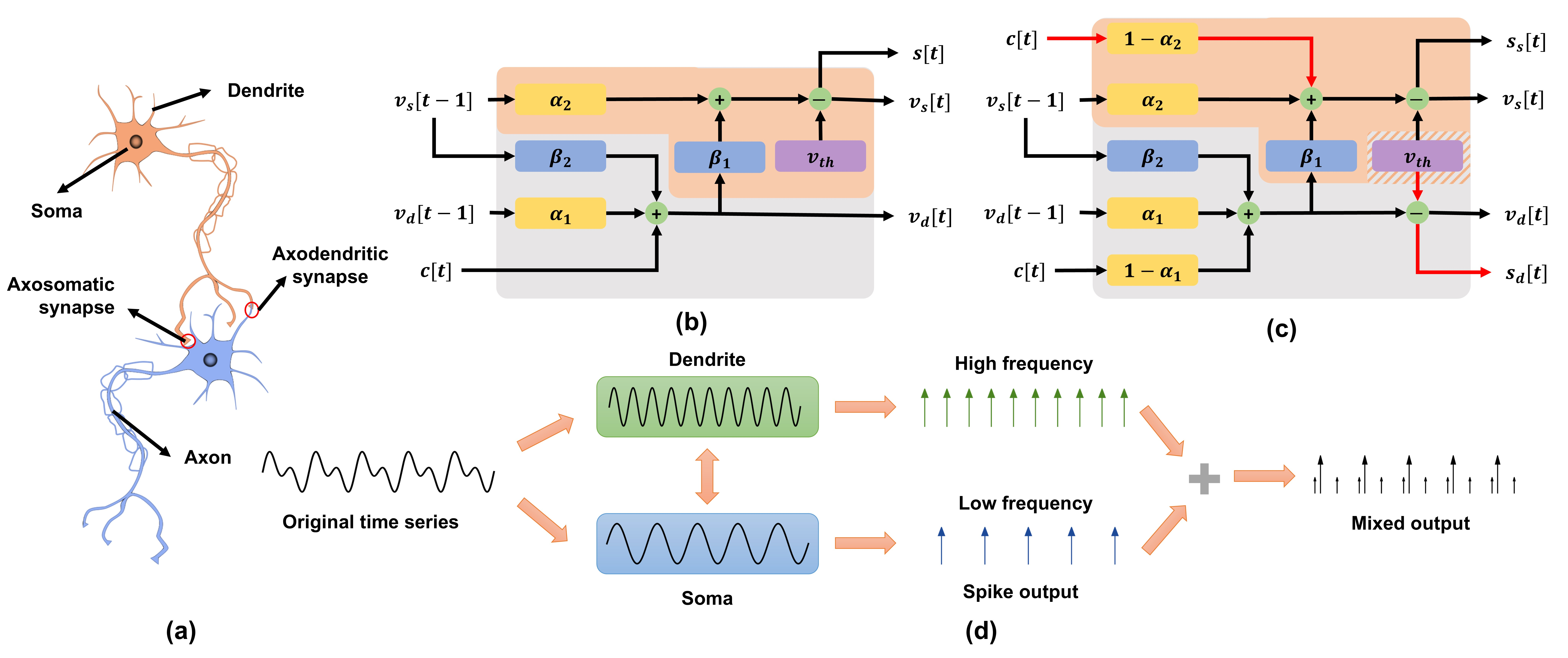
Figure 3. Temporal Segment LIF neuron. The dendritic compartment emphasizes slow and low-frequency components, the somatic compartment captures faster high-frequency responses, and their spike outputs are mixed to improve multi-timescale temporal modeling.
Fourier-Domain Processing: SpikF
A different line of work asks whether attention is necessary at all. SpikF proposes an attention-free spiking Fourier architecture for long-term prediction [8]. The motivation is clear: self-attention can struggle with positional information, while the Fourier transform naturally depends on the order of the sequence through its rotation factors.
SpikF contains three main components. First, a Spiking Patch Encoder splits the input sequence into patches and encodes each patch into binary spike trains. Second, a Spiking Frequency Selector applies S-FFT to grouped spike patches and selects important frequency components. Third, an MLP decoder reconstructs the final continuous-valued forecast.
Because each frequency component depends on all time positions, Fourier-domain processing expands the receptive field and helps long-term dependency modeling. SpikF reports strong long-term forecasting performance, including an average 1.9% MAE reduction compared to state-of-the-art models and a 3.16× lower total energy consumption than iTransformer in the reported energy analysis [8].
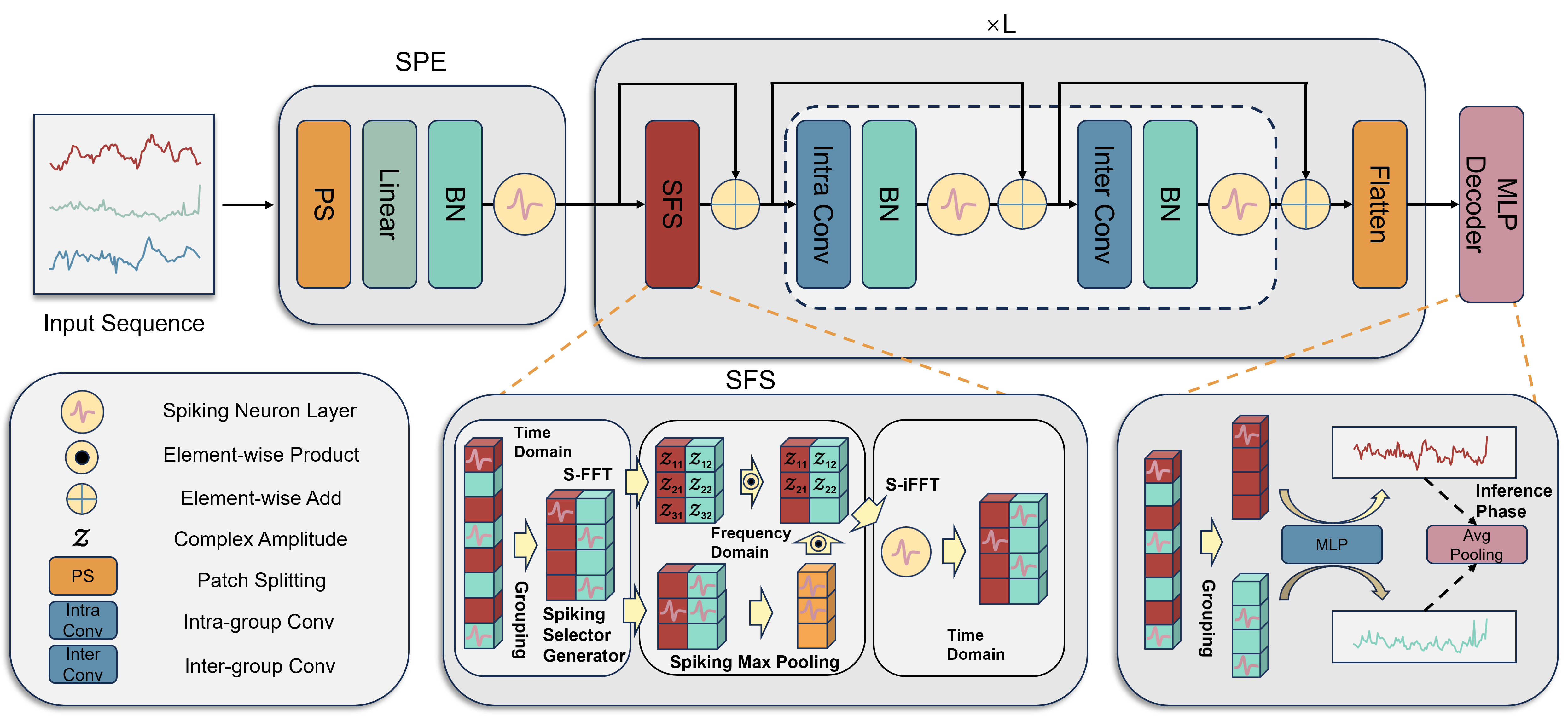
Figure 4. SpikF architecture. The input sequence is divided into patches, encoded as spike trains, processed by S-FFT and spiking frequency selection, and decoded into long-term forecasts.
SpikF is one of the strongest SNN forecasting models, but it still mainly processes variables without an explicit graph structure. In many multivariate forecasting tasks, this is a limitation. Variables are often correlated: traffic sensors influence each other, energy variables co-move, and biomedical signals may contain coupled patterns. Ignoring these relationships leaves useful predictive information unused.
Why Cross-Variable Modeling Matters
Most SNN forecasting models before SpikF-GO focus on temporal dynamics, positional encoding, or neuron design. These are important, but multivariate time series also require cross-variable modeling. If a model processes each variable independently, it can miss correlations between sensors, stations, regions, or channels.
Graph neural networks have been widely used in multivariate forecasting because they can model relationships among variables. However, many graph forecasting models use separate graph modules for cross-variable structure and temporal modules for time dynamics. FourierGNN introduced a hypervariate graph formulation where every scalar observation becomes a graph node [11]. This unifies temporal and variable-level modeling in one structure.
SpikF-GO is built from this idea. It combines the hypervariate graph formulation of FourierGNN with spike-driven Fourier-domain processing inspired by SpikF. The goal is to bring explicit graph-based multivariate modeling into the spiking domain.
SpikF-GO: Spiking Fourier Graph Operators
SpikF-GO treats each scalar observation in the input window as a node [9]. If the input has \(L\) time steps and \(N\) variables, then the hypervariate graph contains:
nodes. This graph can connect any variable at any time step with any other variable at any other time step. In this way, the model can capture three types of information in one representation: intra-series temporal dependencies, inter-series dependencies, and time-varying cross-variable interactions.
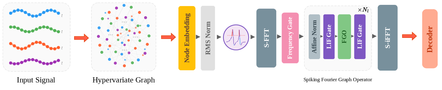
Figure 5. SpikF-GO architecture. The \(L \times N\) input window is represented as a hypervariate graph with \(M=N\times L\) nodes, then processed through S-FFT, a sparse frequency gate, Complex LIF-gated S-FGO layers, S-iFFT, and a decoder for multivariate forecasting.
Encoder and hypervariate graph
The graph formation operator flattens the input:
Each node is projected into an embedding space and normalized. The default model uses RMSNorm, which normalizes without mean subtraction. In our ablation, replacing RMSNorm with a simpler Scale-Shift affine transform gives almost identical performance on Solar and only slight degradation on Traffic and COVID-19, making it a hardware-friendly alternative.
After normalization, the representation is repeated across \(T_s\) SNN steps and modulated by learnable per-step parameters:
A LIF encoder then produces binary spike trains:
S-FFT and sparse frequency gate
SpikF-GO applies S-FFT along the hypervariate graph node axis. In the Fourier domain, multiplication corresponds to graph convolution in the node domain, so spectral operations perform implicit graph mixing:
The model then uses a Hard Concrete frequency gate to learn which frequency bins are useful. During training, a learnable parameter \(\log \alpha_f\) is used for each frequency bin:
The gate is applied to the spectrum:
A sparsity penalty encourages the model to use fewer frequency bins:
This is important for efficiency because fewer active frequencies can reduce computation and make inference more suitable for neuromorphic deployment.
Complex LIF gate and S-FGO block
The S-FGO block applies complex-valued linear operators in the frequency domain. To preserve the event-driven nature of the model, SpikF-GO introduces a Complex LIF gate. For a complex tensor \(Q=Q_r+iQ_i\), the gate applies independent LIF neurons to the real and imaginary parts:
This keeps the spectral computation sparse and binary-gated. After several S-FGO layers, S-iFFT maps the processed spectrum back to the node domain and separates it again into variable and temporal axes:
Decoder
The decoder compresses the temporal dimension, applies a LIF layer at each spiking step, averages over SNN steps, and uses a final projection to produce the forecast. This part returns the model from sparse spike-based processing back to continuous-valued predictions, which are needed for regression tasks such as forecasting.
Main Results of SpikF-GO
SpikF-GO was evaluated on eight multivariate benchmarks under a unified protocol: ECG, COVID-19, Solar, Electricity, METR-LA, Traffic, PEMS-BAY, and Wiki. The baselines include FourierGNN, Spike-GRU, iSpikformer, SpikeRNN/SpikeTCN/Spikformer with CPG, TS-GRU/TS-TCN/TS-Former, and SpikF. The input window and forecast horizon are both 12, and results are averaged over 5 runs [9].
Results on ECG, COVID-19, Solar, and Electricity
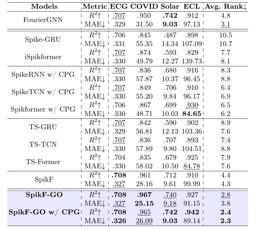
Table 1. Forecasting results on ECG, COVID-19, Solar, and Electricity, averaged over five runs. The table compares FourierGNN and major SNN forecasting baselines with SpikF-GO and SpikF-GO w/ CPG using \(R^2\), MAE, and average rank.
Table 1 shows that SpikF-GO and SpikF-GO w/ CPG are consistently strong. SpikF-GO w/ CPG achieves the best overall average rank on both \(R^2\) and MAE. The CPG variant is especially useful on datasets where additional positional structure improves long-range modeling.
Results on METR-LA, Traffic, PEMS-BAY, and Wiki
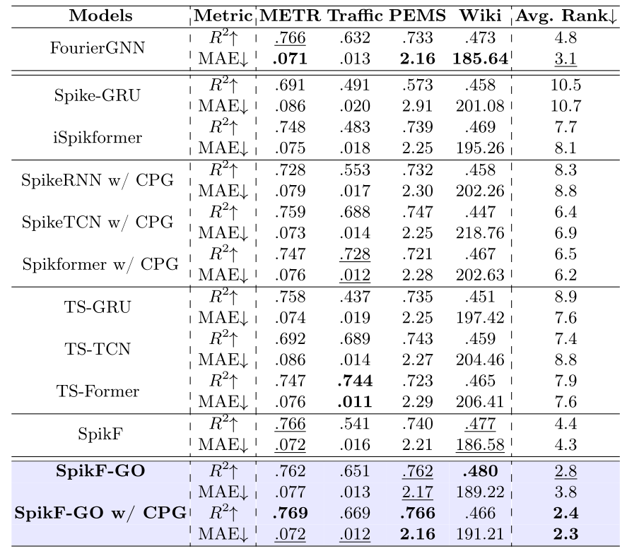
Table 2. Forecasting results on METR-LA, Traffic, PEMS-BAY, and Wiki, averaged over five runs. These datasets are especially important for evaluating cross-variable dependencies in sensor, traffic, and web-traffic forecasting settings.
Table 2 is important because Traffic, METR-LA, and PEMS-BAY contain strong sensor correlations. The improvement of SpikF-GO on these datasets supports the central claim: explicit cross-variable modeling matters for multivariate forecasting.
Hyperparameter sensitivity
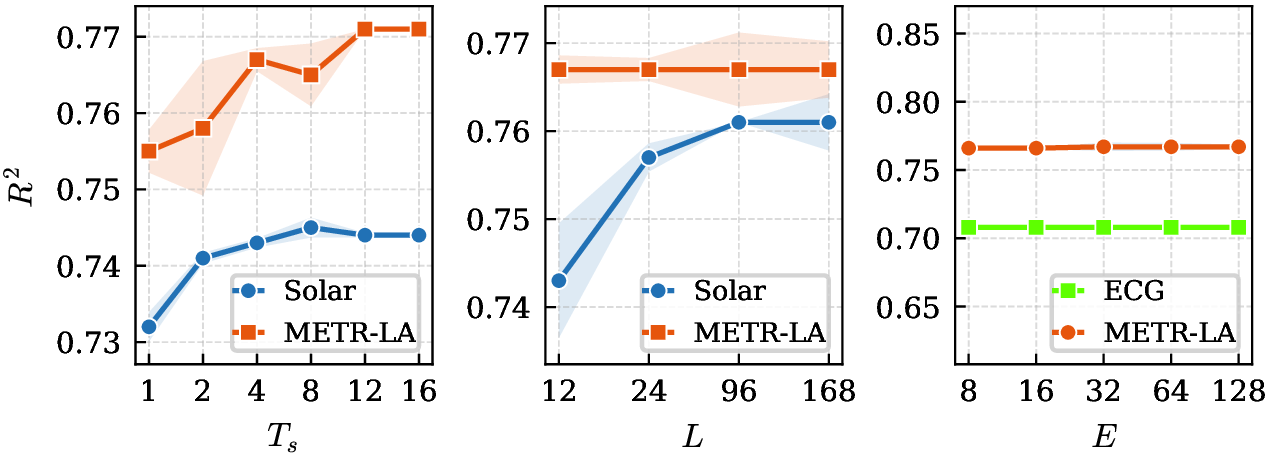
Figure 6. Sensitivity analysis of SpikF-GO with respect to spiking timesteps \(T_s\), input window length \(L\), and embedding size \(E\). Performance improves with more spiking steps until saturation, \(L=96\) is usually sufficient, and compact embeddings can preserve performance while reducing memory and energy cost.
The sensitivity analysis shows that increasing \(T_s\) helps until saturation. Increasing \(L\) beyond 96 gives only small gains in the tested setting. Most importantly, performance remains stable across embedding sizes from \(E=8\) to \(E=128\), which is useful for neuromorphic deployment because smaller embeddings reduce memory and energy cost.
Energy and runtime
| Model | \(E_{\mathrm{Mem}}\) / µJ | \(E_{\mathrm{Ops}}\) / µJ | \(E_{\mathrm{Addr}}\) / µJ | \(E_{\mathrm{Total}}\) / µJ | Time / s |
|---|---|---|---|---|---|
| FourierGNN | \(7.76\times 10^4\) | \(1.13\times 10^4\) | \(1.29\times 10^1\) | \(8.89\times 10^4\) | 0.012 / 0.002 |
| SpikF-GO | \(4.43\times 10^4\) | \(2.17\times 10^3\) | \(5.19\times 10^2\) | \(4.70\times 10^4\) ↓1.89× | 0.027 / 0.011 |
| SpikF | \(2.05\times 10^4\) | \(2.61\times 10^2\) | \(7.91\times 10^1\) | \(2.08\times 10^4\) ↓4.27× | 0.077 / 0.037 |
| SpikF-GO (\(E=8\)) | \(9.28\times 10^3\) | \(2.00\times 10^3\) | \(2.79\times 10^1\) | \(1.13\times 10^4\) ↓7.86× | 0.020 / 0.010 |
Table 4. Energy consumption and wall-clock runtime on Solar with prediction length 12. Energy is decomposed into memory-access, operational, and addressing costs, and reductions are reported relative to FourierGNN.
Table 4 gives the clearest efficiency message. The full SpikF-GO model reduces theoretical energy by 1.89× compared to FourierGNN while improving forecasting performance. The compact \(E=8\) version reaches 7.86× lower energy with little performance change. This is an important result because it shows that graph-based spiking forecasting does not only improve modeling; it can also remain energy-efficient.
There is one practical detail to interpret carefully. FourierGNN has faster wall-clock runtime on GPU because it uses standard ANN operations. SNN models simulate multiple spiking steps on GPU, which introduces overhead. This does not necessarily reflect what would happen on neuromorphic hardware, where spikes can be processed as event-driven operations.
What the Research Direction Shows
Looking across these papers, the story is clear. The first SNN forecasting work showed that spiking versions of TCN, RNN, and Transformer backbones can forecast time series with much lower theoretical energy. CPG-PE showed that positional encoding remains important and can be made spike-compatible. TS-LIF showed that neuron dynamics can be redesigned to better handle long-term and multi-timescale patterns. SpikF showed that Fourier-domain processing is a strong alternative to self-attention for spiking long-term prediction. SpikF-GO then extends this direction to explicit multivariate graph modeling.
The remaining challenge is deployment. Most energy analyses in SNN forecasting papers are theoretical. They use common assumptions such as energy per MAC and energy per AC operation on 45 nm hardware. These comparisons are useful for algorithm design, but future work should test more models on real neuromorphic hardware and include memory access, addressing, and implementation overhead.
Another open direction is the decoder. Forecasting is a regression task, and the final output is usually continuous-valued. This means that even if the encoder and feature extractor are spike-based, the last projection often returns to floating-point values. Building more spike-native decoders for regression is still an important open problem.
Open Library and Future Contributions
To support this growing direction, we maintain SpikingTSF [10], an open-source benchmark library for SNN-based time series forecasting models. The goal is to provide a unified and easy-to-extend library where researchers can compare new SNN forecasting architectures under consistent settings. We welcome new models that are published at conferences, journals, or made available as high-quality preprints, especially models that improve spiking encoders, positional encoding, neuron dynamics, graph modeling, Fourier-domain processing, or neuromorphic deployment.
Conclusion
SNNs bring a different view to time series forecasting. Instead of processing every value with dense continuous operations, they process information through sparse spike events and neuron dynamics. This is attractive for efficient and neuromorphic forecasting, but it also creates new challenges: continuous-to-spike encoding, temporal alignment, positional information, long-term dependency modeling, multivariate correlation modeling, and regression decoding.
The recent progress shows that these challenges are being addressed one by one. Spiking backbones made the first step, CPG-PE improved positional structure, TS-LIF improved neuron dynamics, SpikF showed the power of Fourier-domain processing, and SpikF-GO brings explicit graph-based multivariate modeling into the spiking domain. Together, these works suggest that SNNs can become a serious direction for time series forecasting, especially when efficiency and deployment constraints matter.
References
- W. Maass. Networks of Spiking Neurons: The Third Generation of Neural Network Models. Neural Networks, 1997.
- J. K. Eshraghian et al. Training Spiking Neural Networks Using Lessons from Deep Learning. arXiv:2109.12894, 2023.
- K. Yamazaki, V.-K. Vo-Ho, D. Bulsara, and N. Le. Spiking Neural Networks and Their Applications: A Review. Brain Sciences, 2022.
- A. L. Hodgkin and A. F. Huxley. A quantitative description of membrane current and its application to conduction and excitation in nerve. Journal of Physiology, 1952.
- C. Lv, Y. Wang, D. Han, X. Zheng, X. Huang, and D. Li. Efficient and Effective Time-Series Forecasting with Spiking Neural Networks. ICML, 2024.
- C. Lv, D. Han, Y. Wang, X. Zheng, X. Huang, and D. Li. Advancing Spiking Neural Networks for Sequential Modeling with Central Pattern Generators. NeurIPS, 2024.
- S. Feng, W. Feng, X. Gao, P. Zhao, and Z. Shen. TS-LIF: A Temporal Segment Spiking Neuron Network for Time Series Forecasting. ICLR, 2025.
- W. Wu, D. Huo, and H. Chen. SpikF: Spiking Fourier Network for Efficient Long-term Prediction. ICML, 2025.
- J. Bakhshaliyev and N. Landwehr. SpikF-GO: Spiking Fourier Graph Operators for Multivariate Time Series Forecasting. In: Ceci, M., et al. Machine Learning and Knowledge Discovery in Databases. Research Track. ECML PKDD 2026. Lecture Notes in Computer Science, vol. 16943. Springer, Cham, 2027. doi.org/10.1007/978-3-032-37664-0_3. Also on arXiv:2606.13901. Code: github.com/jafarbakhshaliyev/SpikF-GO.
- J. Bakhshaliyev. SpikingTSF: A Unified Benchmark Library for Spiking Neural Network Based Time-Series Forecasting. GitHub repository, 2026. github.com/spikora/SpikingTSF.
- K. Yi, Q. Zhang, W. Fan, H. He, L. Hu, P. Wang, N. An, L. Cao, and Z. Niu. FourierGNN: Rethinking Multivariate Time Series Forecasting from a Pure Graph Perspective. NeurIPS, 2023.
- S. Bai, J. Z. Kolter, and V. Koltun. An Empirical Evaluation of Generic Convolutional and Recurrent Networks for Sequence Modeling. arXiv:1803.01271, 2018.
- K. Cho et al. Learning Phrase Representations using RNN Encoder–Decoder for Statistical Machine Translation. EMNLP, 2014.